FEM of J-integral
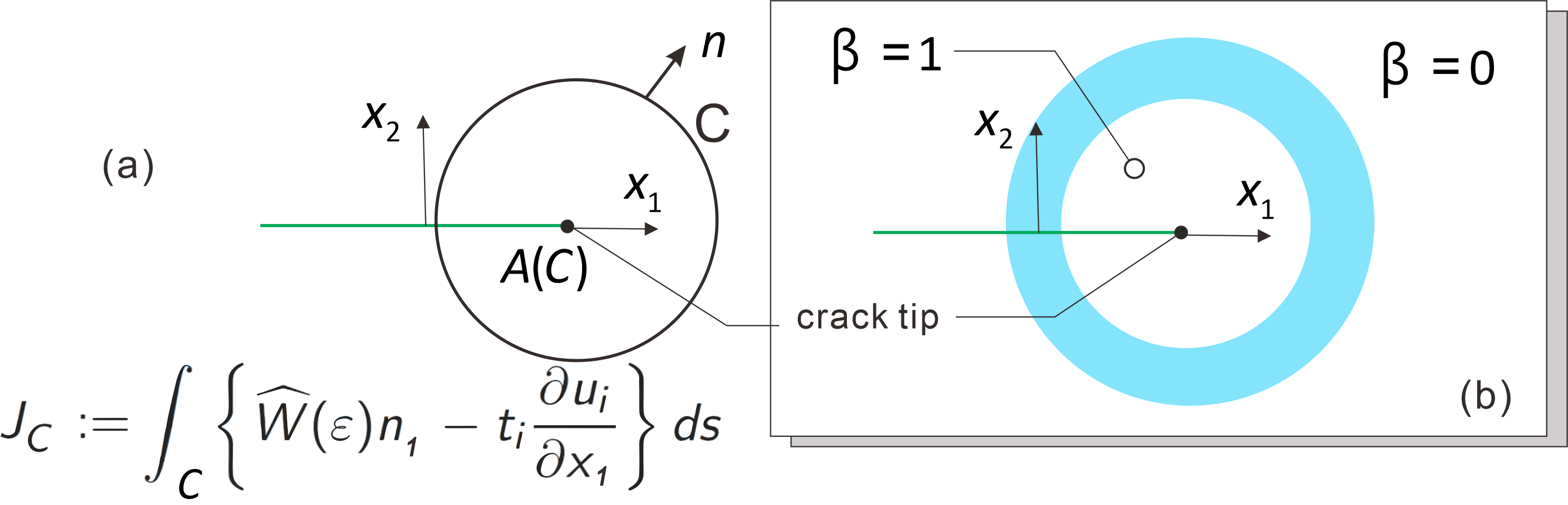
(a) J-integral defined on a path C (b) G-theta integral
Here we notice that $\int _{A(C)}\partial \widehat{W}(\varepsilon )/\partial x_1~dx=\infty $. So that (3.A2) and (3.A3) does not hold near the crack tip,
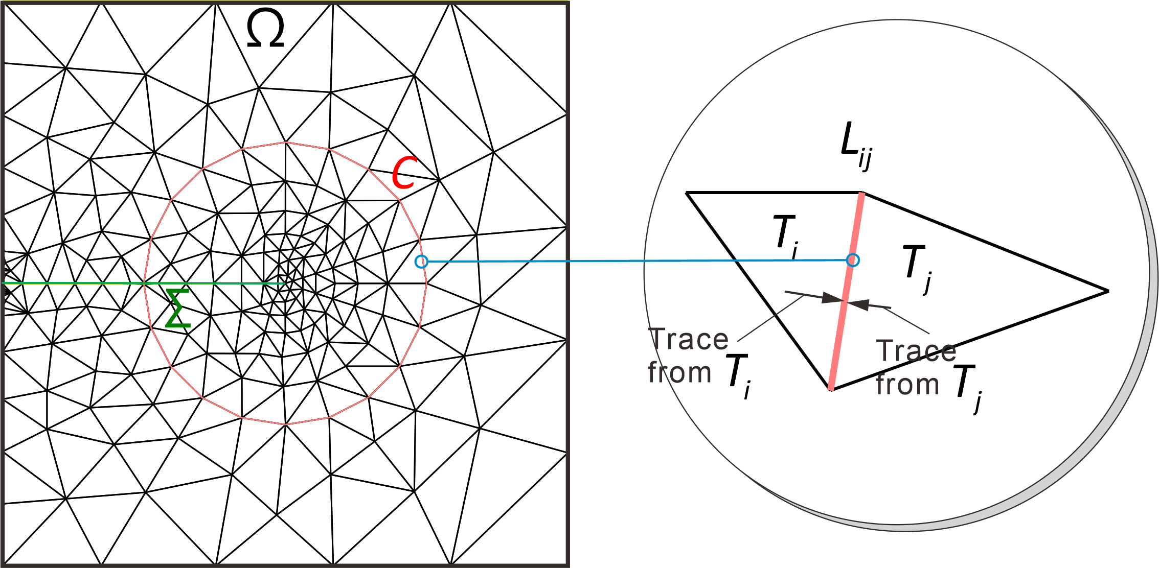
Triangulation of the domain $(-1,1)^2\setminus \Sigma $ and the path $C$ and the trinangles $T_i,T_j$ near $L_{ij}\subset C$ The crack is approximated by a narrow notch.
When J-integral depend on path
When the body force $f\neq 0$ at the crack tip, the J-integral is not path independent and must be $\lim _{C→0}J_C$, but with the GJ-integral, the following holds even if $f\neq 0$ \begin{eqnarray*} R_{\omega }(u,\mu ) &=&-\int _{\omega \cap \Omega }\left \{ \frac{1}{2}(\mu \cdot \nabla C_{ijkl})e_{kl}(u)e_{ij}(u)+f_{i}(\nabla u_{i}\cdot \mu )\right . \\ &&-\left . \sigma _{ij}(u)\partial _{j}\mu _{k}\partial _{k}u_{i}+ \frac{1}{2}\sigma _{ij}(u)e_{ij}(u)\textrm{div}\mu \right \} dx \end{eqnarray*} Or we can use the relation \begin{eqnarray*} \mathcal{G}(u,f,\Sigma (\cdot ))&:=&J_C+R_{A(C)}(u,e_1)\\ R_{A(C) }(u,e_1 ) &=&-\int _{A(C)\setminus \Sigma }\left \{ \frac{1}{2} (\partial _1C_{ijkl})e_{kl}e_{ij}+f_{i}(\partial _1 u_{i})\right \} dx \end{eqnarray*}FreeFEM
PDEs have been developed with the aim of understanding natural phenomena. Until 2000, there was a large gap between theoretical research on mathematical models and numerical simulation. FreeFEM , which has been developed by F. Hecht, led by O. Pironneau at Laboratoire Jacques-Louis Lions , is considered to bridging the gap between theory and computation. Hereafter, from this point of view, concrete FE-calculations are shown using FreeFEM.FreeFEM Examples
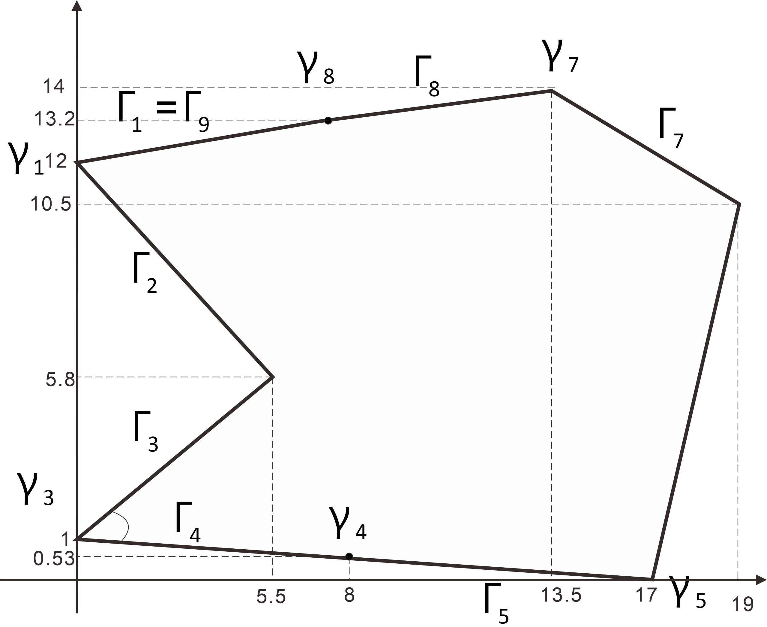
The polygonal domain shown in the example
real[int] px=[   8, 0,5.5,0,   8,17,  19,13.5];
real[int] py=[13.2,12,5.8,1,0.53, 0,10.5,  14];
/* ---------- Define boundary $\Gamma _1...\Gamma _8$---------- */
border Gm1(t=0,1){x=(1-t)*px[0]+t*px[1];y=(1-t)*py[0]+t*py[1];}
border Gm2(t=0,1){x=(1-t)*px[1]+t*px[2];y=(1-t)*py[1]+t*py[2];}
border Gm3(t=0,1){x=(1-t)*px[2]+t*px[3];y=(1-t)*py[2]+t*py[3];}
border Gm4(t=0,1){x=(1-t)*px[3]+t*px[4];y=(1-t)*py[3]+t*py[4];}
border Gm5(t=0,1){x=(1-t)*px[4]+t*px[5];y=(1-t)*py[4]+t*py[5];}
border Gm6(t=0,1){x=(1-t)*px[5]+t*px[6];y=(1-t)*py[5]+t*py[6];}
border Gm7(t=0,1){x=(1-t)*px[6]+t*px[7];y=(1-t)*py[6]+t*py[7];}
border Gm8(t=0,1){x=(1-t)*px[7]+t*px[0];y=(1-t)*py[7]+t*py[0];}

real mh = 5; /* Number of mesh divisions */
mesh Th = buildmesh(Gm1(mh)+Gm2(mh)+Gm3(mh)+Gm4(mh)+Gm5(mh)
                    +Gm6(mh)+Gm7(mh)+Gm8(mh));
plot(Th,bw=1,wait=1);
Connecting the points (px[i],py[i]) and (px[i+1],py[i+1]) and dividing $mh$, the enclosed area is automatically triangulated.
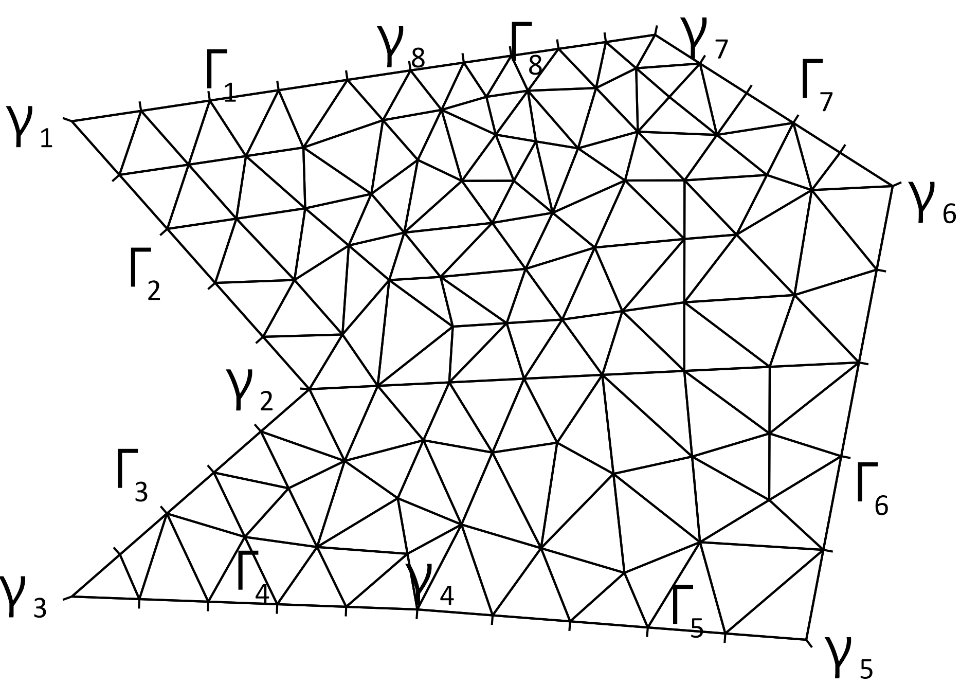
The triangulation of the polygonal domain
Poisson problem with Dirichlet boundary condition
Now we calculate Poisson Problem: $-\Delta u=f$ in $\Omega $ with the Dirichlet boundary condition. Redefine the boundary with boundary conditions./* ---------- Define boundary ---------- */ int bcD=2, bcN=3; //To give boundary conditions func real cnt(real[int] p, int i, real t) { int j = ((i+1)>7) ? 0 : i+1; return (1-t)*p[i]+t*p[j]; } border Gm1(t=0,1) { x=cnt(px,0,t);y=cnt(py,0,t);label=bcD;} border Gm2(t=0,1) { x=cnt(px,1,t);y=cnt(py,1,t);label=bcD;} border Gm3(t=0,1) { x=cnt(px,2,t);y=cnt(py,2,t);label=bcD;} border Gm4(t=0,1) { x=cnt(px,3,t);y=cnt(py,3,t);label=bcD;} border Gm5(t=0,1) { x=cnt(px,4,t);y=cnt(py,4,t);label=bcD;} border Gm6(t=0,1) { x=cnt(px,5,t);y=cnt(py,5,t);label=bcD;} border Gm7(t=0,1) { x=cnt(px,6,t);y=cnt(py,6,t);label=bcD;} border Gm8(t=0,1) { x=cnt(px,7,t);y=cnt(py,7,t);label=bcD;} real mh = 5; /* Number of mesh divisions */ mesh Th = buildmesh(Gm1(mh)+Gm2(mh)+Gm3(mh)+Gm4(mh)+Gm5(mh) +Gm6(mh)+Gm7(mh)+Gm8(mh));Now, we define FE-space with P1-elements, and create the FE-approximation $u_h$ and test function $v_h$
/* Define FE-space with P1-element */
fespace Vh(Th,P1);
Vh u,v; /* FE-solution and Test function */
Next, the variational form \begin{eqnarray*} \textrm{Poisson}(u_h,v_h):&&\int _{\Omega }\left (\frac{\partial u_h}{\partial x}\frac{\partial v_h}{\partial x}+\frac{\partial u_h}{\partial y}\frac{\partial v_h}{\partial y}\right ) dx-\int _{\Omega }f_vh dx=0\\ &&\textrm{with }u_h=0~~~\textrm{on }\Gamma _i~~\textrm{labelled bcD} \end{eqnarray*} of the Poisson problem is created as follows.
func f = 1; // f(x,y)=1

problem Poisson(u,v) =
        int2d(Th)( dx(u)*dx(v) + dy(u)*dy(v))
        - int2d(Th)( f*v )
        + on(bcD,u=0);
At this point, approximate solution $u_h$ is not computed. When computing simultaneously, solve is used instead of problem . However, if solve is used, the variational form Poisson cannot be re-used. Finally, the variational form Poisson is solved and the iso-lines (contours) are plotted.
Poisson; // Solve the Poisson
plot(u,value=true,wait=1); // Iso value of u
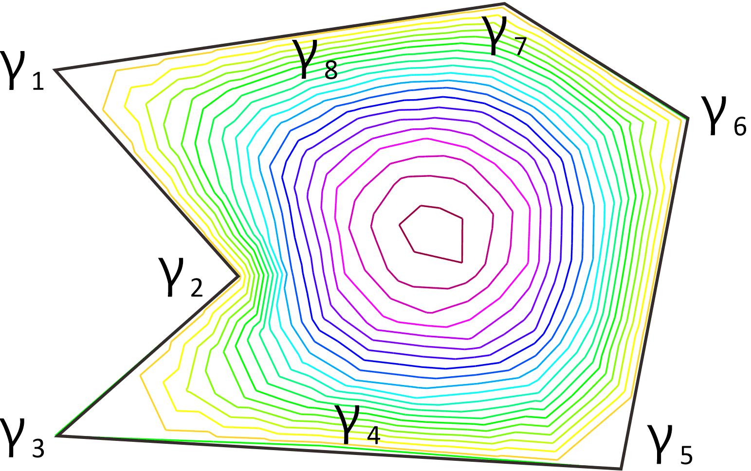
The iso-lines of Poisson Problem with Dirichlet boundary condition
Poisson problem with Mixed boundary condition
Now solve the mixed boundary given in example . It can be solved by simply changing the labels on the boundaries.border Gm5(t=0,1) { x=cnt(px,4,t);y=cnt(py,4,t);label=bcN;} border Gm6(t=0,1) { x=cnt(px,5,t);y=cnt(py,5,t);label=bcN;} border Gm7(t=0,1) { x=cnt(px,6,t);y=cnt(py,6,t);label=bcN;} border Gm8(t=0,1) { x=cnt(px,7,t);y=cnt(py,7,t);label=bcN;}
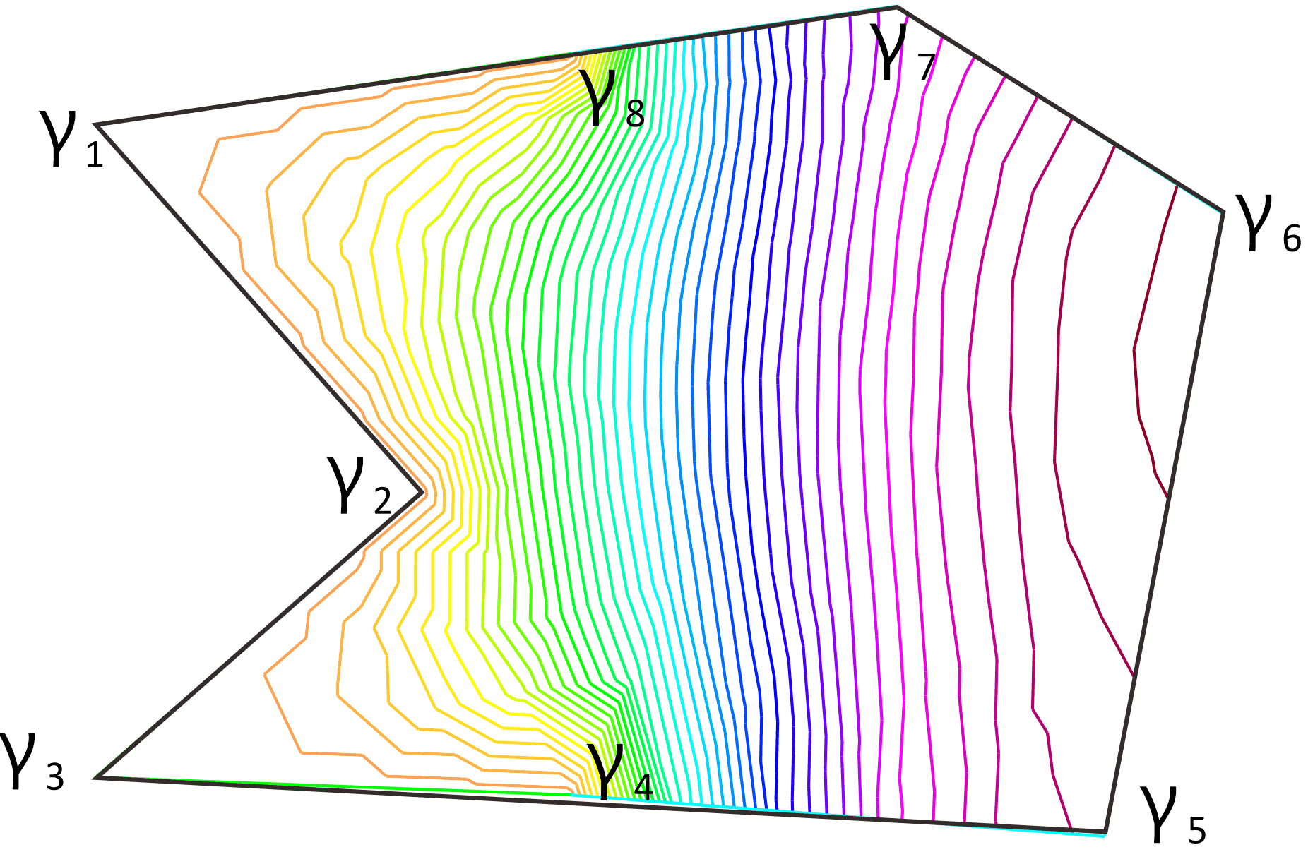
The iso-lines of Poisson Problem with Mixed boundary condition
Th = adaptmesh(Th,u);
plot(Th,wait=1);
Poisson; // Solve the Poisson
plot(u,nbiso=40,wait=1); // Iso value of u
.
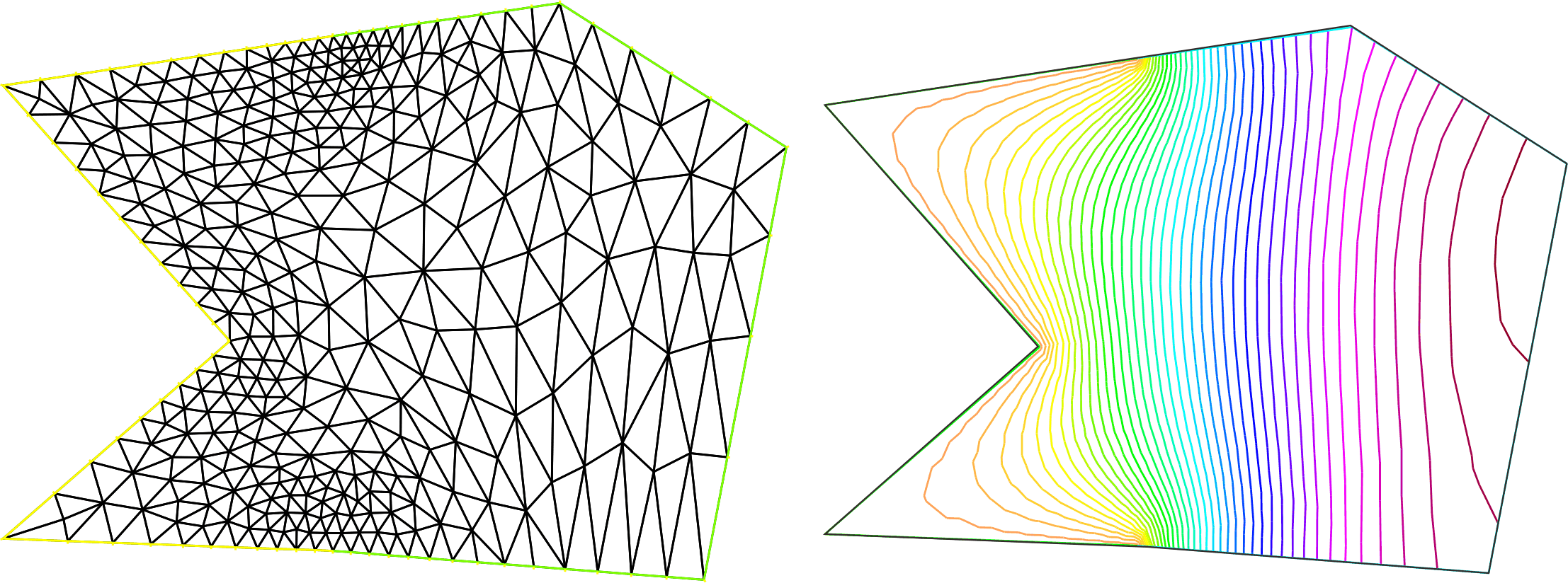
The mesh and iso-lines after using adaptmesh
for (int i=0; i<5; i++) {
  Th = adaptmesh(Th,u);
  Poisson; // Solve the Poisson
}
plot(Th,wait=1);
plot(u,nbiso=40,wait=1); // Iso value of u
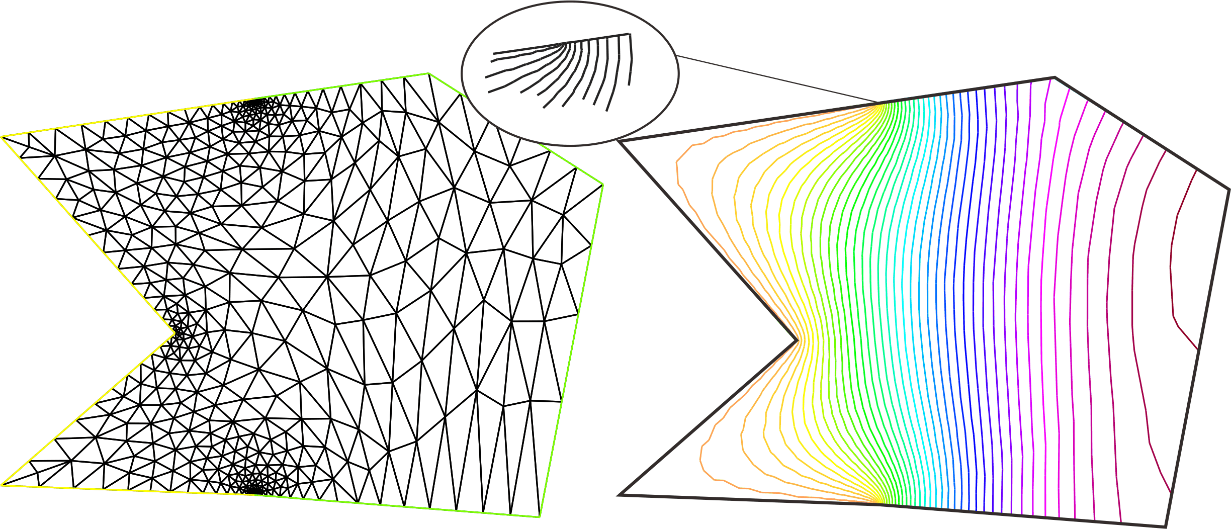
After repeated adaptmesh, the mesh and the iso-line
Energy sensitivity at singular point
There are strong singular points $\gamma _4, \gamma _8$ and weak singular point $\gamma _3$. In general, energy has no sensitivity in the tangential direction of the boundary[Th.2.27, Sok92], but in mixed boundary problems there is a sensitive in the tangential direction at junctions $\{\gamma _4,\gamma _8\}$. We now measure the shape sensitivity at $\gamma _8, p_2=(11,13.63), p_1=(5,12.74)\in \Gamma _8$ using $$ R_{\Omega }(u,\tau (\gamma _8)\beta (\gamma _8)), R_{\Omega }(u,\tau (\gamma _8)\beta (p_i)), i=1,2$$ where $\tau $ is the tangential vector and $\beta (p), p\in \Gamma _8$ at cut-off function near $p$ (see Theorem Poisson with mixed boundary ). Here $\tau (\gamma _8)∼-(0.989,0.146)$. From Corollary 2.9 , we have \begin{eqnarray*} \left .\frac{d}{dt}\mathcal{E}(u(t);f,\Omega (t))\right |_{t=0} &=&-R_{\Omega }(u(t),\mu _{\varphi })-\int _{\partial \Omega }fu(n\cdot \mu _{\varphi })\\ &&~~\mu _\varphi =d\varphi _t/dt|_{t=0} \end{eqnarray*} Now introduce the cut-off function $\textrm{be}(x_1,x_2,c_1,c_2,r)$ such as $$ \textrm{be}=1~\textrm{if }rr \lt r^2;=0~\textrm{if }rr \gt 4r^2; =2-\sqrt{rr}~\textrm{if }r^2 \lt rr \lt 4r^2$$ where $rr=|x_1-c_1|^2+|x_2-c_|^2$. By the mapping $\varphi _t(x)=x+t\tau (\gamma _8)\beta _1(x)$, $\beta _1=\textrm{be}(x_1,x_2,8,13.2,1)$, $\varphi _t(\Omega )=\Omega $ but $\varphi _t(\Gamma _8)\neq \Gamma _8$. Using the cut-off functions $\beta _1=\textrm{be}(x_1,x_2,8,13.2,1)$, the mapping $\varphi _t(x)=x+t\tau (\gamma _8)\beta _1(x)$, and then from Theorem Poisson Mixed boundary $$ \left .\frac{d}{dt}\mathcal{E}(u(t);f,\Omega )\right |_{t=0} =R(u,\tau (\gamma _8)\beta _1)=\frac{\pi }{8}K(\gamma _8)^2 \gt 0$$ To calculate $R(u,\mu \beta )$. we prepare the following function $$ \textrm{Rin}(v,\beta ,\mu _1,\mu _2):= -f(\nabla u\cdot (\beta \mu ))+\nabla u\cdot \nabla (\beta \mu _k)\partial _k u-0.5|\nabla u |^2\textrm{div }(\beta \mu )$$ In FreeFEM, the functions be and Rin are implemented using func and macro .func real be(real xx, real yy, real cx, real cy, real r) { real rr = (xx-cx)^2+(yy-cy)^2; if (rr< r^2) return 1; else i f (rr > 4*r^2) return 0; else return 2-sqrt(rr); } macro Rin(uu,cut,Xx,Xy) ( -f*(Xx*dx(uu)+Xy*dy(uu))*cut + ((cut*dx(Xx)+dx(cut)*Xx)*dx(uu) + (cut*dy(Xx)+dy(cut)*Xx)*dy(uu))*dx(uu) + ((dx(cut)*Xy+cut*dx(Xy))*dx(uu) +(dy(cut)*Xy+cut*dy(Xy))*dy(uu))*dy(uu) - 0.5*(dx(uu)*dx(uu)+dy(uu)*dy(uu)) *(dx(cut)*Xx+dy(cut)*Xy+cut*(dx(Xx)+dy(Xy))) ) //and $\beta _1,\beta _2,\beta _3$ are created as follows
Vh beta = be(x,y,8,13.2,1);
Vh beta2 = be(x,y,5,12.74,1);
Vh beta3 = be(x,y,11,13.63,1);
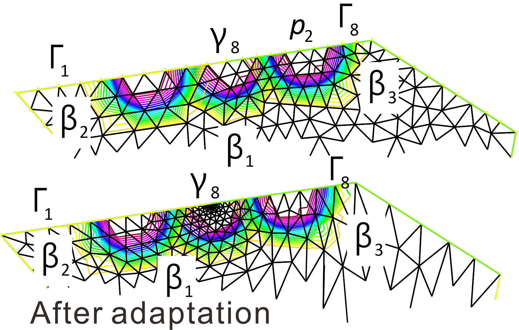
iso-line of FE-approximations beta,beta2,beta3 of $\beta _1, \beta _2,\beta _3$
Poisson; // Solve the Poisson
real Rint = int2d(Th)(Rin(u,beta,Xx,Xy));
real Rint2 = int2d(Th)(Rin(u,beta2,Xx,Xy));
real Rint3 = int2d(Th)(Rin(u,beta3,Xx,Xy));
cout <<"R-integral=" << Rint << ", @(5.12.74) " << Rint2
                     <<", @(10,13.48) "<< Rint3 << endl;
The results are as follows
R-integral=318.863, @(5.12.74) 0.675089, @(10,13.48) 0.757448After adaptation of mesh using adaptmesh , we obtain
R-integral=325.187, @(5.12.74) 0.222543, @(10,13.48) -0.379611By numerical calculation, we have that sensitivity exist at $\gamma _8$ in the tangential direction, but no sensitivity at $p_1,p_2$ in the tangential direction because $\varphi _t(\Gamma _1)=\Gamma _1$ if $\varphi _t(x)=x+t\beta _2\tau (\gamma _8)$, $\varphi _t(\Gamma _8)=\Gamma _8$ if $\varphi _t(x)=x+t\beta _3\tau (\gamma _8)$.