What's SoptS
The theme is named SoptS (Shape Optimisation of Singular Points in BVPs) to study fracture phenomena and (boundary) shape optimisation in terms of singularity of solutions of boundary value problem for partial differential equations (BVPs). Core studying SoptS is the generalised J-integral (GJ-integral), which is based on the J-integral of fracture mechanics.
(MaKR = Mathematical Knowledge Repository, making since around 2000.)
The main topics are more details and additional pictures of AMS-SoptS
Finite element analysis and shape optimization of singular points in boundary value problems for partial differential equations
published in the journal Sugaku Expositions
from American Mathematical Society
Topics
- Mathematical research based on the concept of fracture mechanics starting from graduate school (1980), that is a really difficult problem and has not been solved yet.
- I proposed a gneralization (GJ-integral) of J-integral to express 3-dimensional fracture phenomena in 1981
- Systematic study of shape sensitivity analysis such as Hadamard's variational formula using GJ-integral.
- The method using GJ-integral has features such as being applicable even if the boundary value problem has singular points and also extracting local features
Fracture
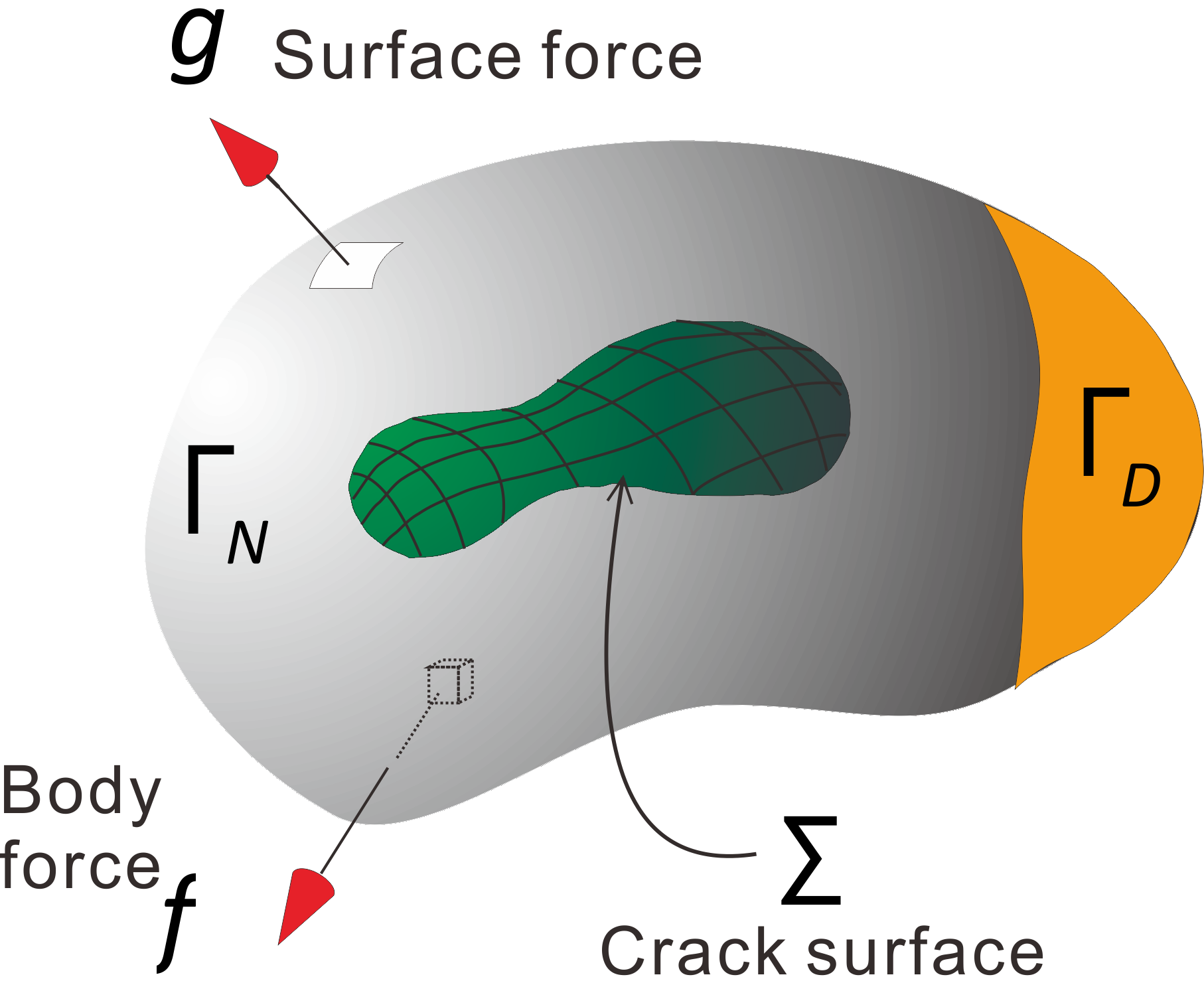
Let $\Omega $ be a bounded domain with Lipschitz boundary in $\mathbb{R}^d, d=2,3$, and $\Sigma \subset \Omega $ be a surface with the edge. The elasticity is defined on the domain $\Omega _{\Sigma }:=\Omega \setminus \Sigma $ with stress free $\sigma _{ij}^{±}(u)\nu _j=0$ on $\Sigma $,where $u$ is the displacement permitting the jump across the crack , $\sigma _{ij}^{±}(u)$ the stress on the both($±$) side of $\Sigma $, and $\nu =(\nu _j)_{j=1,…,d}$ is the unit normal vector on $\Sigma $ directed from the plus side toward the minus. Notice that $u^+(x)=u^-(x)$ on $x\in \partial \Sigma $.Examining the singularity at the edge of the crack in an elastic body with a crack is called crack problem.
Shape Optimization of boundary
Let $\Omega $ be a bounded domain with Lipschitz boundary in $\mathbb{R}^d, d=2,3$ and $u(\Omega )$ a minimizer of an energy functional $\mathcal{E}$ over a subset $V(\Omega )$ in the function space $W^{1,p}(\Omega ;\mathbb{R}^m),m\ge 1$, Consider a cost functional $F(u(\Omega ))$. The shape optimization of boundary is a problem of finding a method of deforming a given set $\Omega $ so as to lower the cost function, and optimized shape $\Omega ^O$ is given by $$ F(u(\Omega ^O)) \lt F(u(\Omega ))$$
Energy Optimization in Dirichlet boundary conditions
A famous example is the Poisson's equation $-\Delta u=f$ with Dirichlet boundary conditions; $u=0$ on $\partial \Omega $. The minimizer $(u^{OD},\Omega ^{OD})$ of the energy $\mathcal{E}(u)=\int _{\Omega }\{|\nabla u|^2/2-fu\} dx$, that is, $$ F(u(\Omega ^{OD}))=\min _{\Omega }\{F(u(\Omega )):|\Omega |=constant\}$$ satisfy the condition $\partial u^{OD}/\partial n=\textrm{constant}$ on $\partial \Omega ^{OD}$. Here $F(u(\Omega ))=\mathcal{E}(u)$. The figure just below is the numerical example when $f=1$.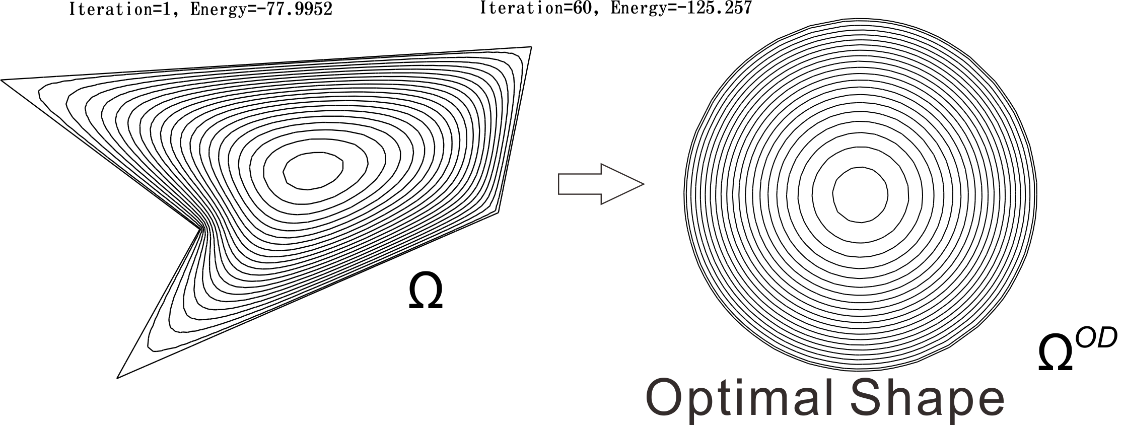
Optimal design $\Omega ^{OD}$ obtained by iterative calculation from the polygon on the left
Just because the disk $\Omega ^{OD}$ is energy stable, not all shapes can be made into a disk. It is more practical to think about how to deform the shape to make it more energy stable. We say Shape Optimization Problem to find the method how to deform the shape $\Omega $ to make more stable shape $\Omega ^{O}$. We call $\Omega ^O$ optimized shape, and $\Omega ^{OD}$ (if exists) is called optimal shape (right hand side of the figure just above).
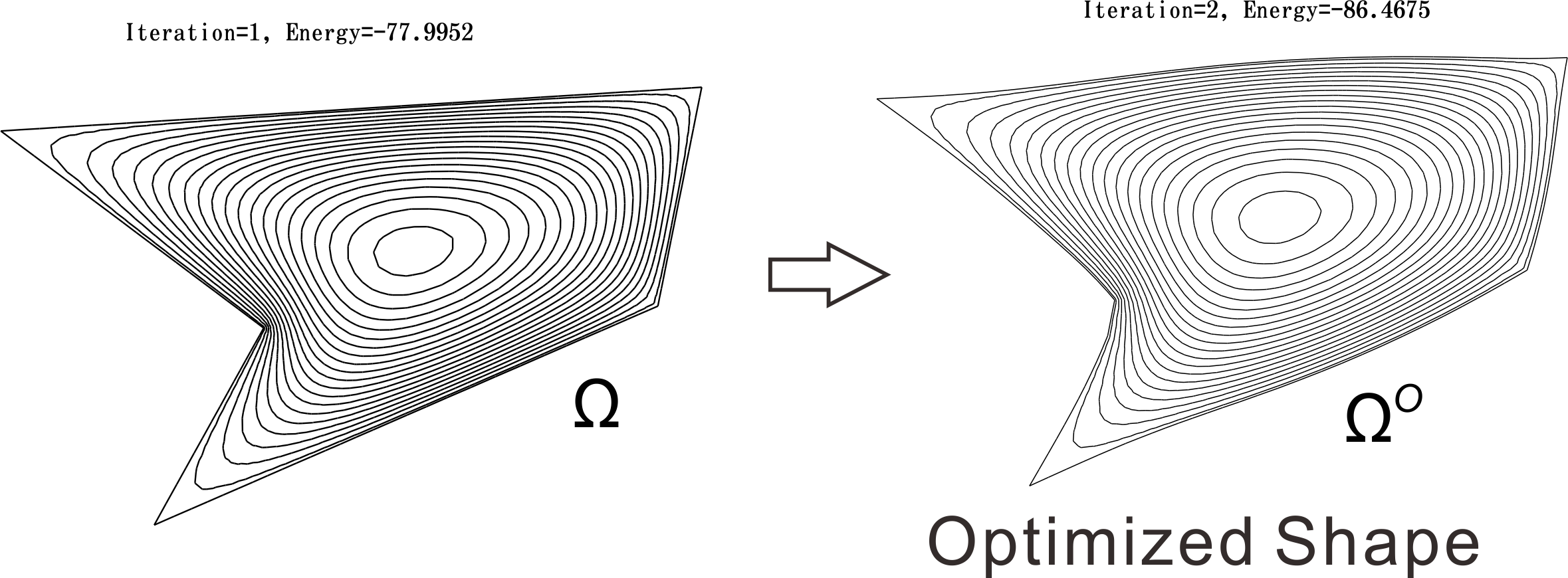
An optimized shape of a polygonal domain
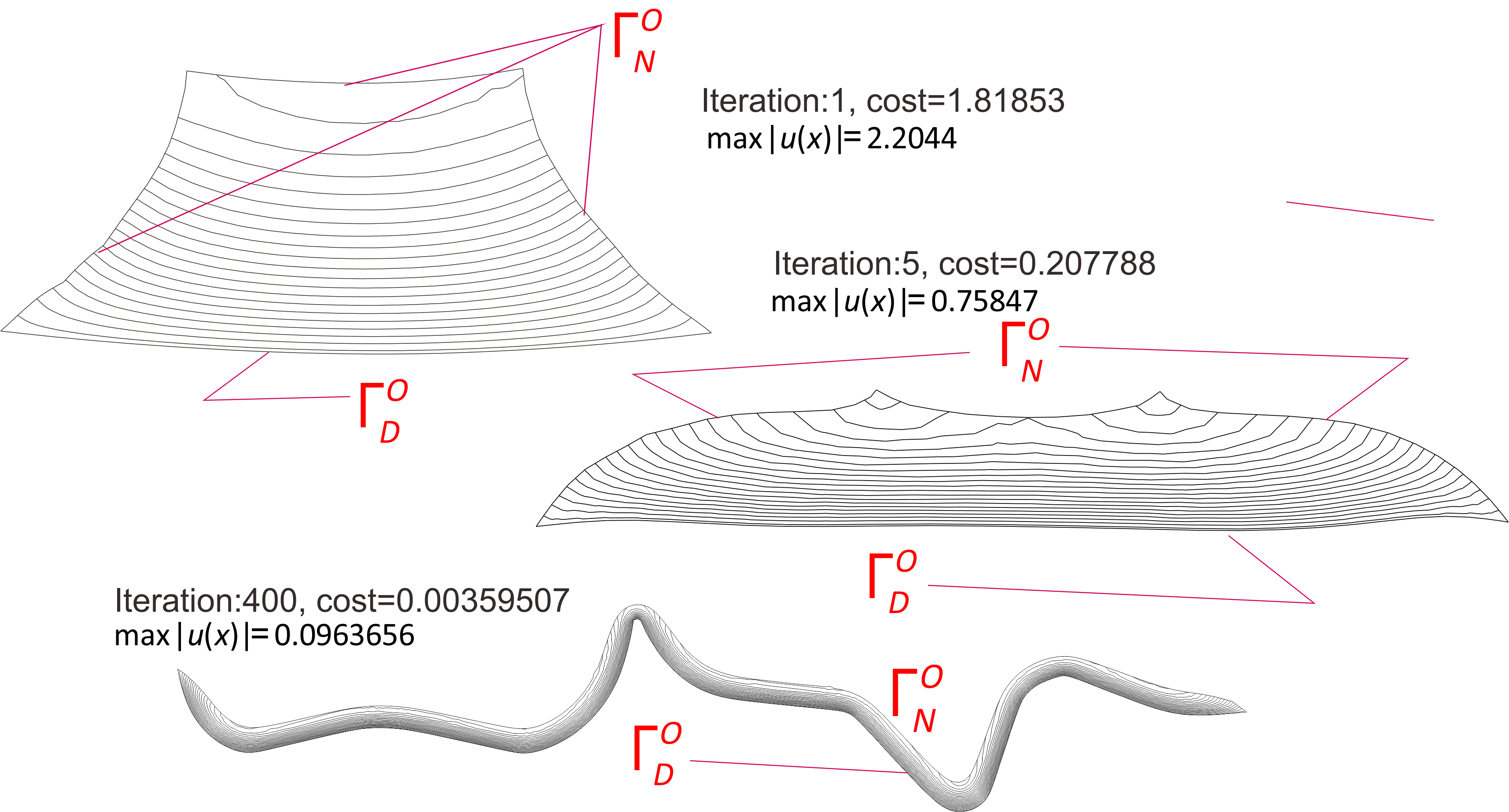
Optimization in Mixed boundary condition
Select the unit disk $\Omega =\{(x_1,x_2):x_1^2+x_2^2 \lt 1\}$ as the initial, $u=0$ on $\Gamma _D=\partial \Omega \cap \{x_2 \gt 0\}$ and put $\partial u/\partial n=0$ on $\Gamma _N=\partial \Omega \cap \{x_2 \lt 0\}$ as shown in the figure just below. The right figure is an optimized shape $\Omega ^O$ of $\Omega $. The solution $u$ has high singularity at $\gamma _M^i,i=1,2$, that is, $u\notin H^{3/2}$ and $u\in H^{3/2-\epsilon }$ near $\gamma _M^i,i=1,2$ for all $\epsilon \gt 0$.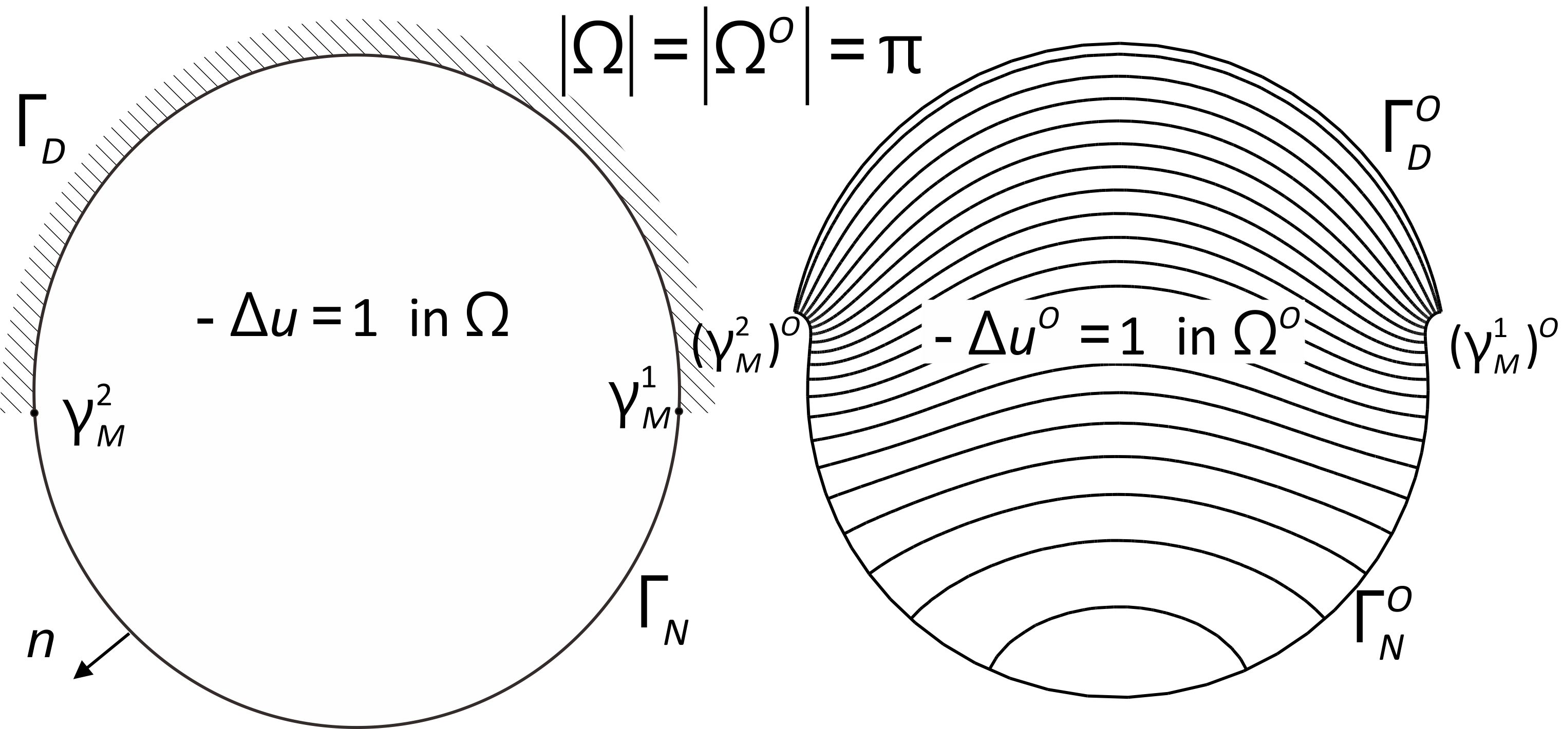
Optimized shape in Poisson Eq. with mixed boundary condition
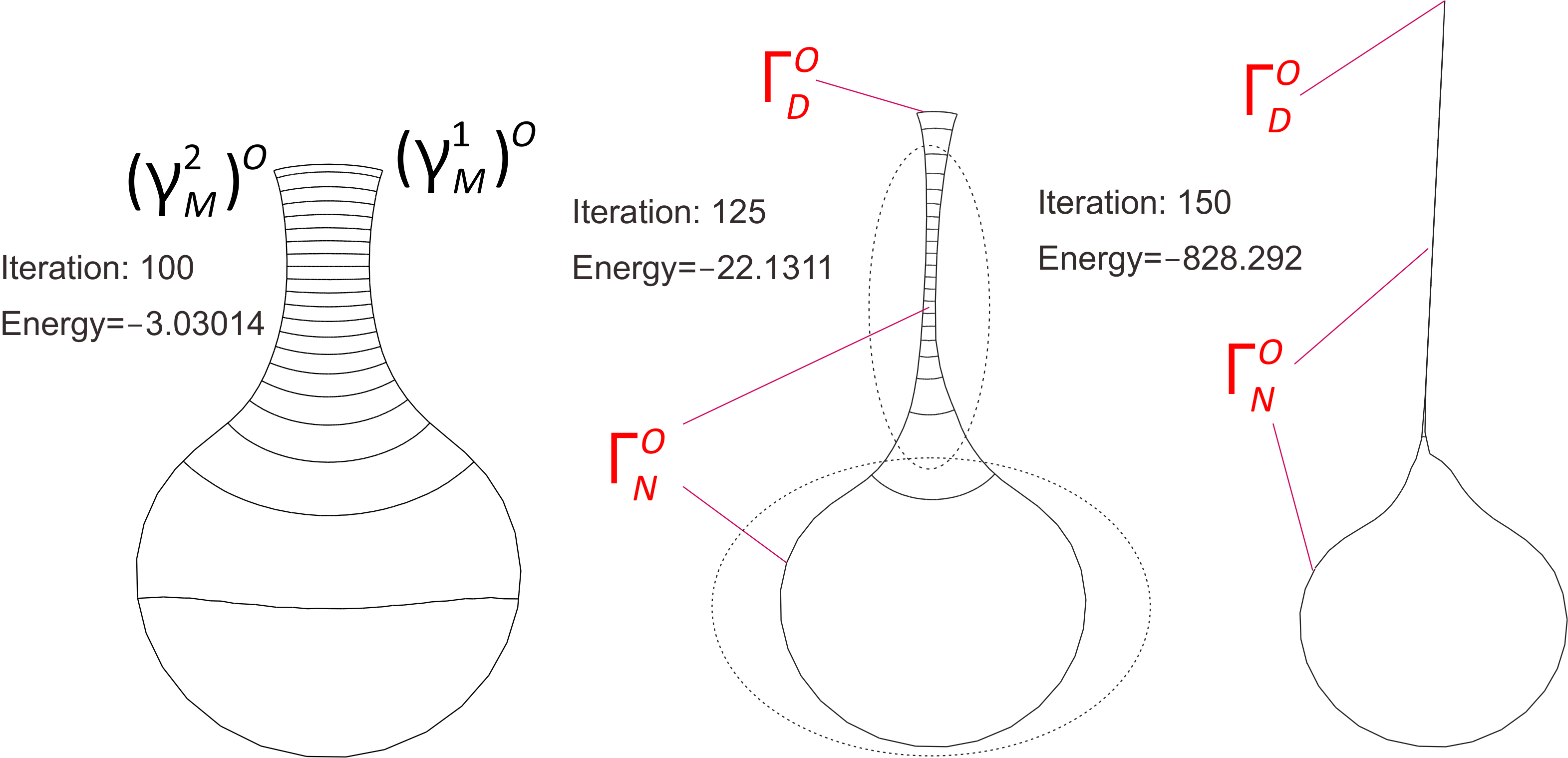
A series of optimizations can be obtained.
$\Gamma _D^O$ become small like a dot, and $\Gamma _N^O$ has a shape in which a thread is attached to a disk and connected to $\Gamma _D^O$.
Notice that optimized shapes are determined by $f$ in $-\Delta u=f$. For example $f(x_1,x_2)=\sin (2\pi x_1)$, we get a series of optimized shapes as shown below..
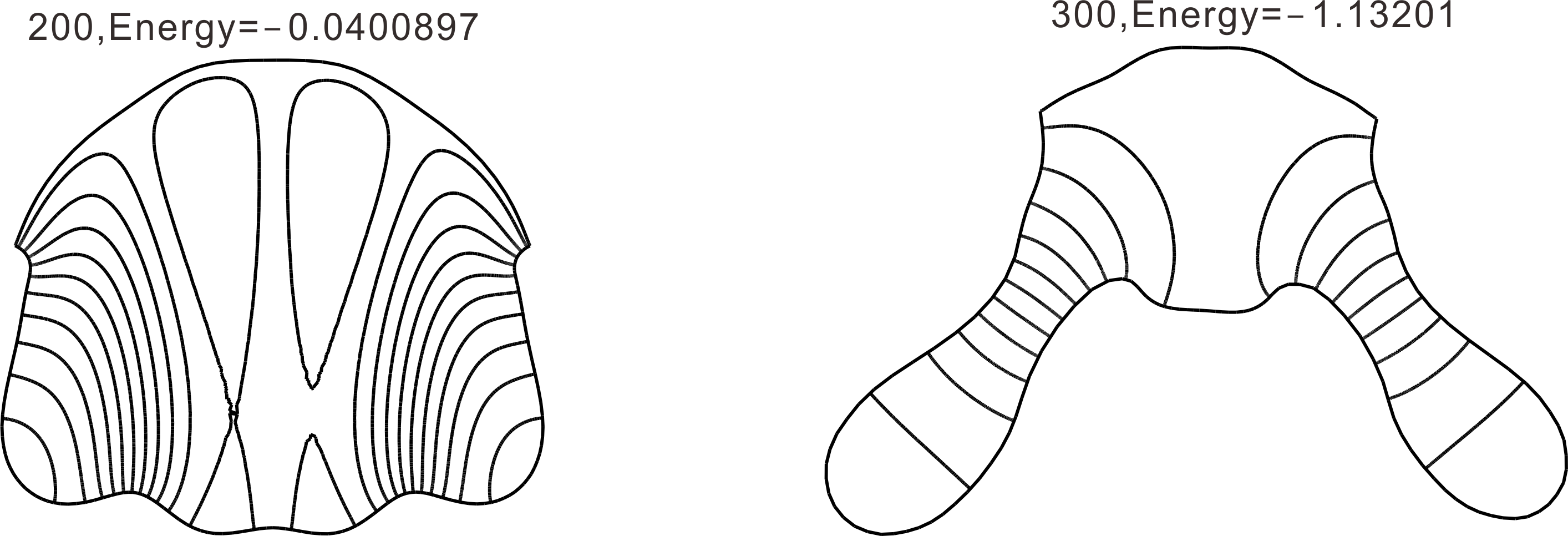
A series of optimizations under $-\Delta u=\sin (\pi x_1)$.
Mean Compliance Optimization
Cantilever by Allaire (see [Al07] 6.5 Algorithmes numériques) More..The initial domain $\Omega $ is just below. A series of domains $\Omega ^O_k$ satisfying the constraints $|\Omega ^O_k|=\textrm{constant}$ ($|D|$ represents the area of D.). $$ F(\Omega )=\int _{\Gamma _N}g\cdot u\,ds$$
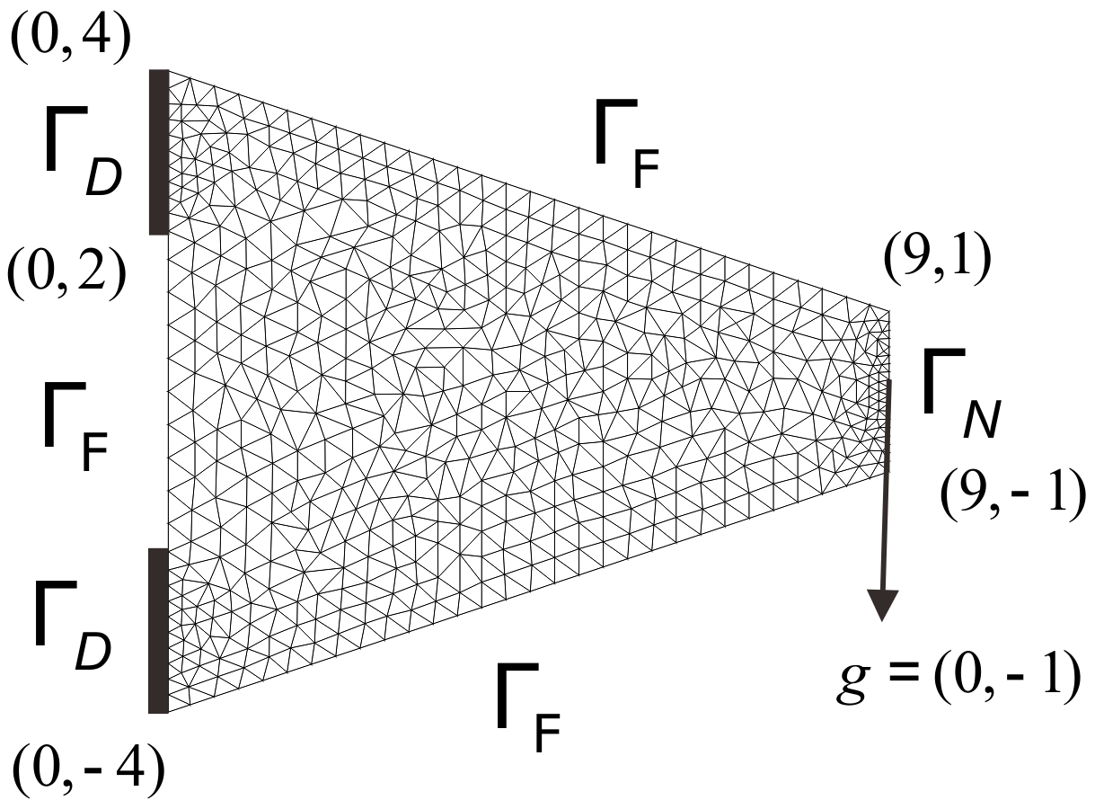
where $\Gamma _N$ is fixed and vertical deformation of $\Gamma _D$ B is allowed. In [Al07], $\Gamma _D$ is fixed.
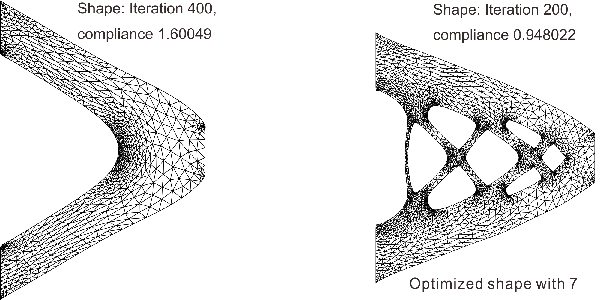
The left side is the optimized shape in the figure just above, and the right side is the optimized shape with 7 holes.
More..
Least Square Error
For a given functoin $u_d$, find $(u^O,\Omega ^O)$ such that $$ F(u(\Omega )):=\int _{\Omega }|u(\Omega )-u_d|^2dx$$ The example below is an optimized shape when $u_d = 0$ in Poisson's equation under Dirichlet boundary conditions starting from the square region. Since it corresponds to the problem of cooling, it is considered that the longer the boundary, the more optimized domains.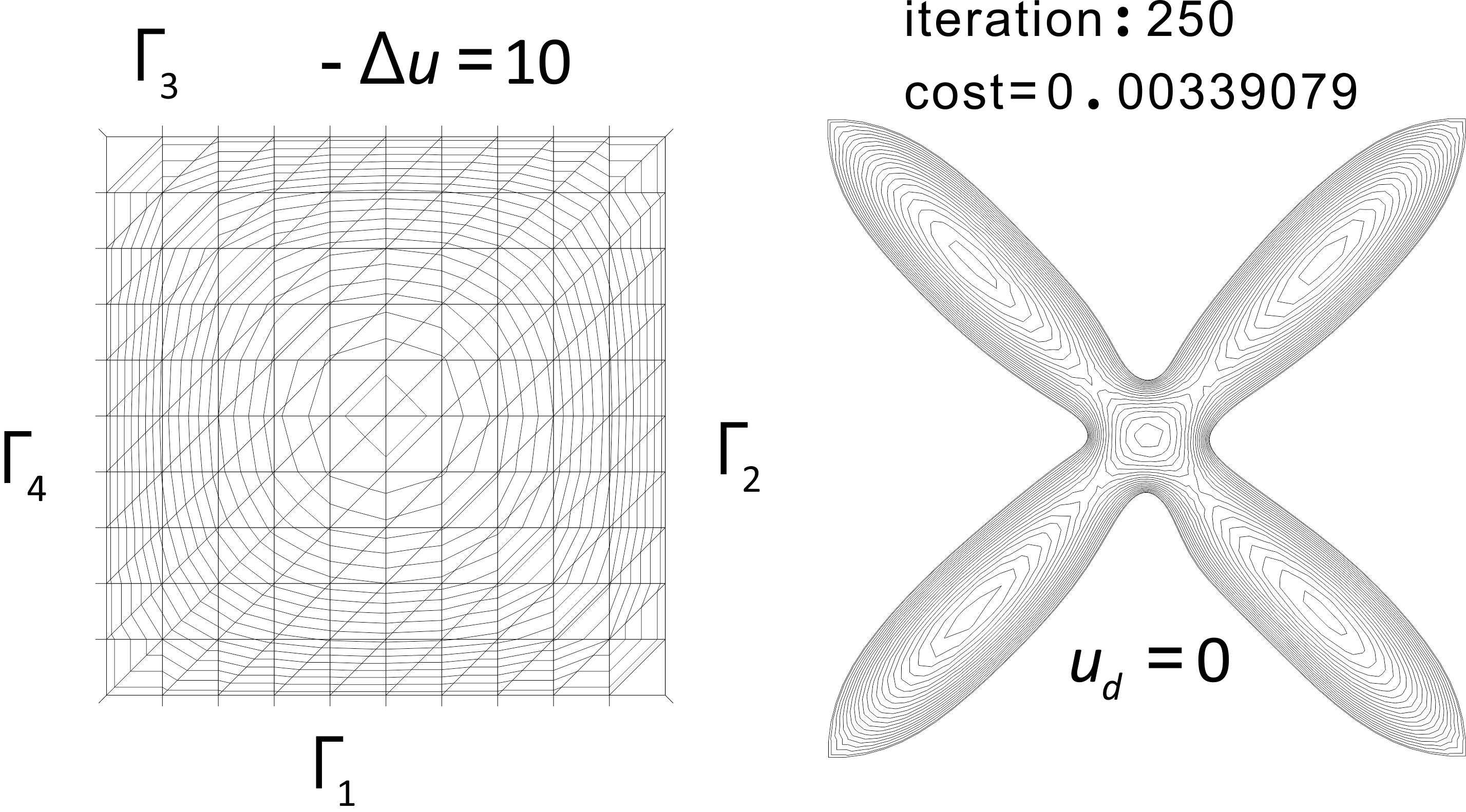
The left side is the starting region, and an optimized domain in the right.
At the 400th iteration, the optimized shape looks like an elongated string.
Shape optimization of Interfaces
Consider a composite in which two different elastic plates are joined together. The static shape is divided into $\Omega _1$ and $\Omega _2$ as shown on the left in the figure below, and Young's modulus are $E_1 = 200, E_2=20$ and Poisson's ratio are $\nu _1=0.25, \nu _2=0.3$. The initial compliance is $14.2113$ and the compliance after optimization is $12.092$ as shown in the figure on the right.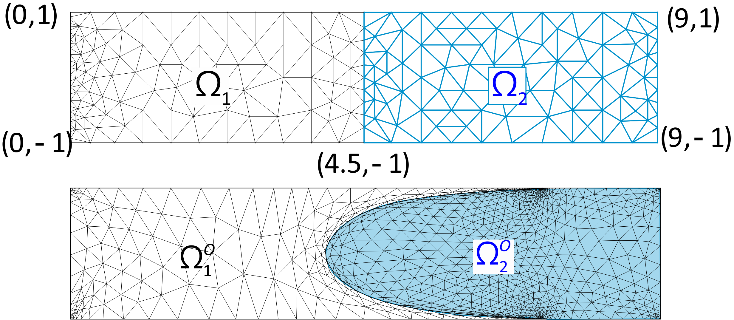
Acknowledgments
In fracture mechanics, it was helpful to have the discussion in CoMFoS (Continuum Mechanics Focusing Singularities); in particular to, S.Aoki, Y.Sumi, C.Yatomi, T.Nishioka, K.Kishimoto, S.Hirose, M.Hori. CoMFoS was created in 1995 by T.Miyhoshi, C.Yatomi and myself as a group for theoretical research on fracture mechanics, and in 2004 it became the activity group of the Japanese Society for Applied Mathematics. From a mathematical perspective, it was useful to discuss with members in CoMFoS;in particular, T.Miyoshi, N,Nishimura, H.Ito. Collaborators are: M.Kimura on non-linear problems (Theorem 2.10 ); A.M.Khludnev and J.Sokolowski on the development of GJ-integral; V.Kovtunenko on the Lagrange multiplier method . I am indebted to provid research environment abroad; W.L.Wendland in Stuttgart, O.Pironneau and F.Hecht at FreeFEM project in France. For teaching me functional analysis in graduate school, Hiroshima University; F.Maeda, A.Inoue, M.Tetsuro, K.Yoshida. In Shape Optimization, H.Azegami, with his H1-gradient method , paved the way from sensitivity analysis to shape optimisation, and the numerical results using FreeFEM were encouraging.